Mathematica is one of the last programs I would use to create a figure for publication. However, it can still be useful to know how to make a nice looking plot in Mathematica. If you are manipulating equations and data in Mathematica, it’s useful to be able to generate a decent looking plot until you have settled on your final viewing angle and parameter values without exporting the data numerous times.

Basic Parameters

A lot of parameters can be used in most types of graphics objects, sometimes with minor tweaks to the name or input objects.

Labeling

Plot Labels

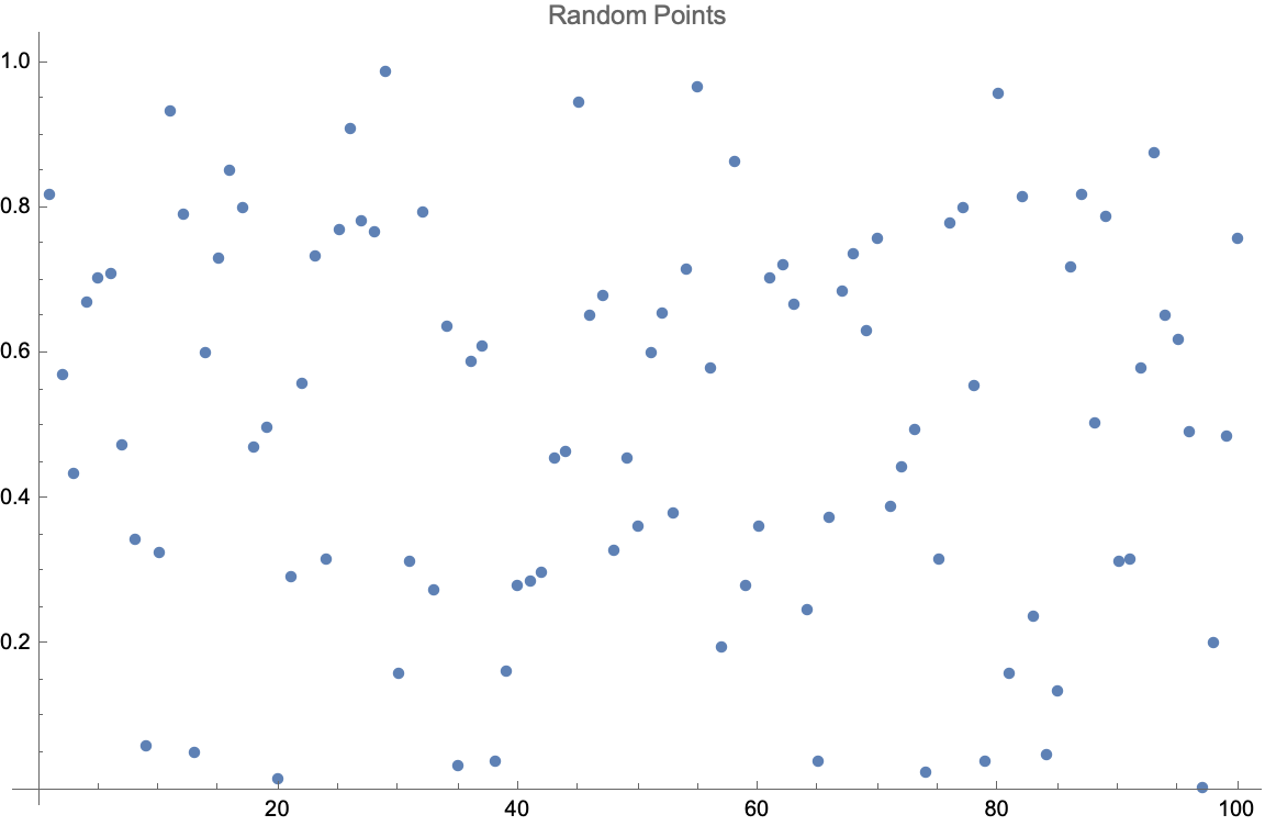
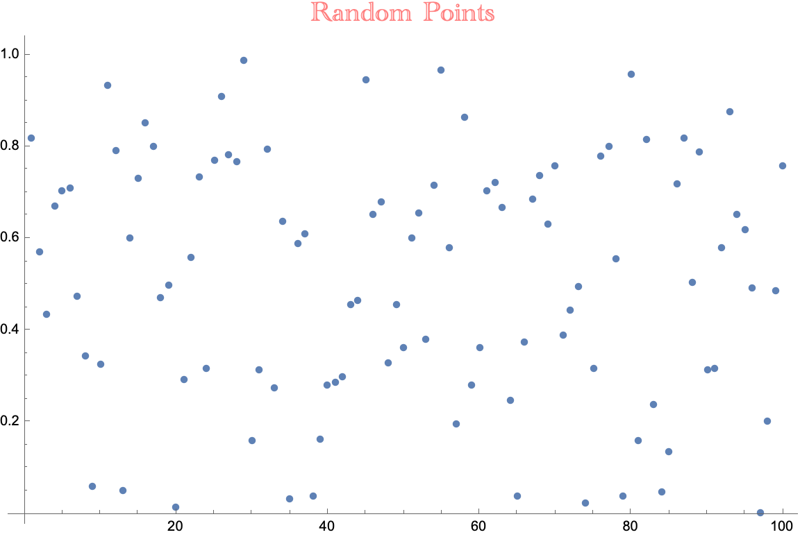
The basic way to add an overall label to a plot is using the argument PlotLabel -> "Plot Name!". This generates a basic title with a default font size, style, and typically in a faint grey colour. We can gain more control over these aspects of the plot label by using the Style function. For example:

x = Range[1,100];
y = RandomReal[{0,1},100]; (* Generate 100 random real numbers between 0 and 1 *)
data = Transpose[{x,y}]; (* Create an (x,y) list of points for plotting *)

ListPlot[data, PlotLabel -> "Random Points", ImageSize -> Large]	ListPlot[data, PlotLabel -> Style["Random Points", Pink, 20, FontFamily -> "Academy Engraved LET"], ImageSize -> Large]

The ImageSize option is used here to generate nicely sized plots for exporting. Note that most style aspects of your plot will not scale with the size of the plot. Make sure that you set this parameter to a value you like before messing around too much with the size of style elements.

Axes Labels

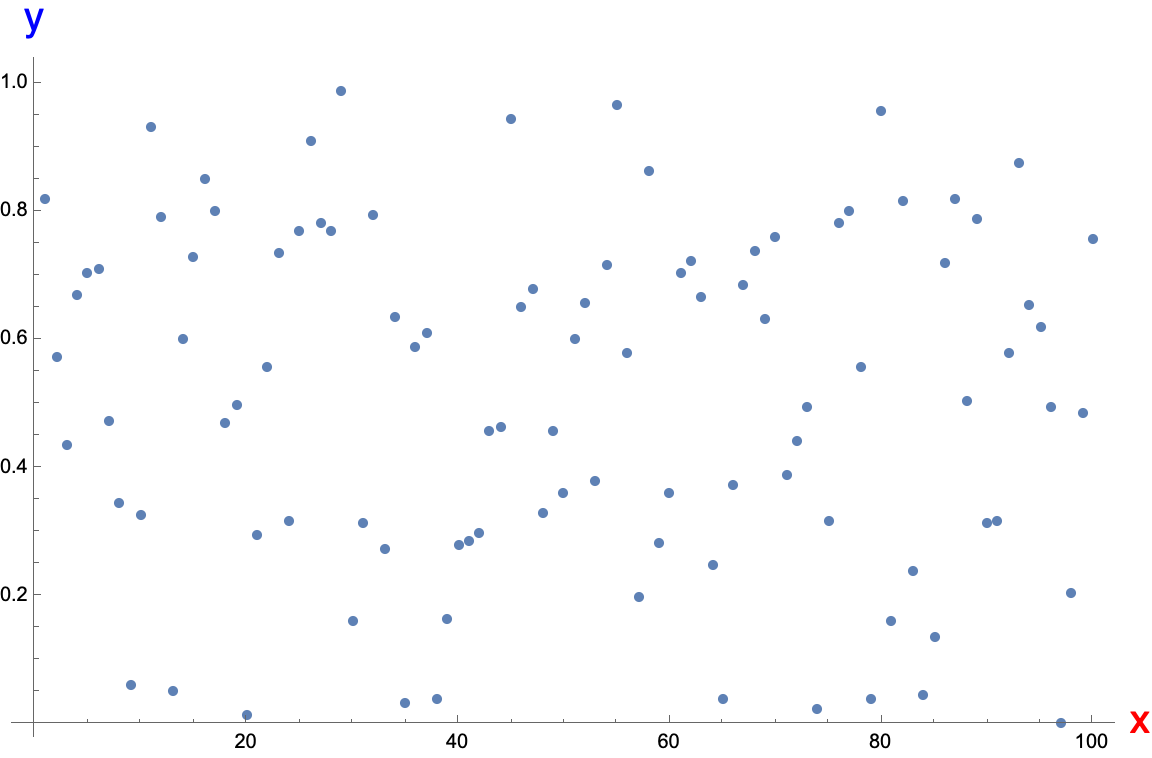
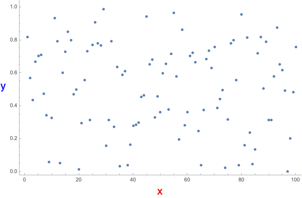
AxesLabel is the basic way to label the axes of your plot. Like PlotLabel you can pass a simple set of strings, i.e. AxesLabel -> {"x","y"}, or enhance the style using the Style function as in the below example. FrameLabel is a more complex option to generate axes labels, but also offers more fine-tuning and better placement. To use FrameLabel we also need to supply the Frame argument. Frame takes as its input a Boolean or set of Booleans that decides whether a frame is drawn on the graphics object. True draws an edge on every side of the graphics object. Or you can give a nested list with the arguments in the order of {left, right} and then {bottom,top}. FrameLabel takes its input in the same format and order, replacing the Booleans with a Style function or string or the parameter None to leave the edge unlabeled. By default, the left and right labels are rotated by 90 degrees, which I have undone with the Rotate function in the below example.

ListPlot[data, AxesLabel -> {Style["x", 20, Red, FontFamily -> "Helvetica"], Style["y", 20, Blue, FontFamily -> "Helvetica"]}, ImageSize -> Large]	ListPlot[data, Frame -> {{True, False},{True,False}}, FrameLabel -> {{Style[Rotate["y",90 Degree], 20, Blue, FontFamily -> "Helvetica"], None},{Style["x", 20, Blue, FontFamily -> "Helvetica"], None}}, ImageSize -> Large]

Plot Legends

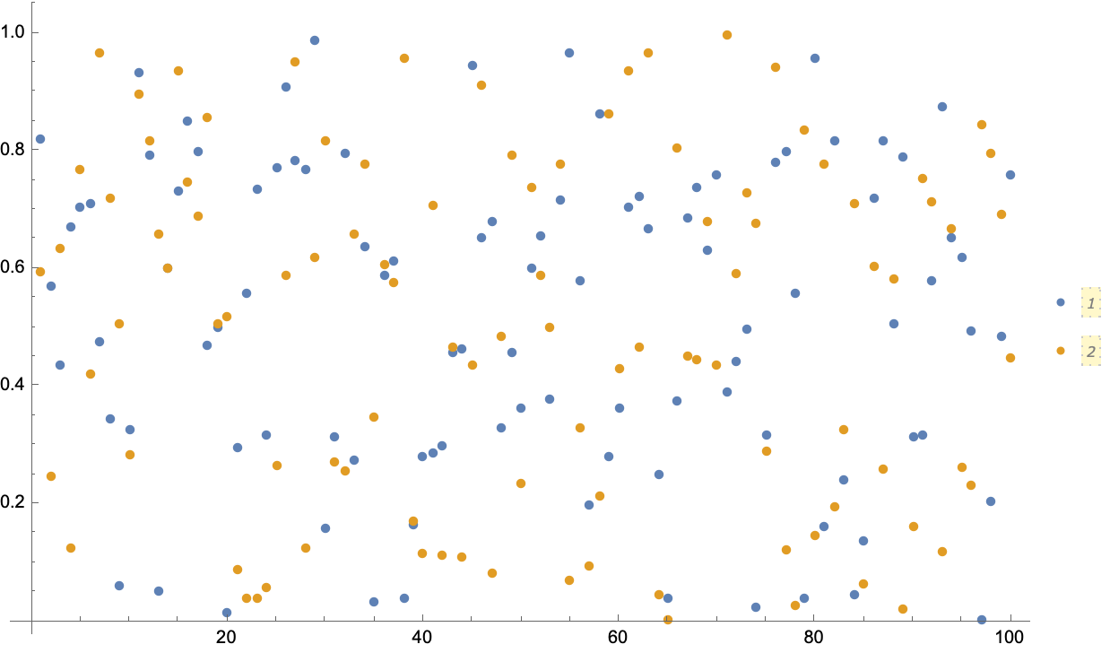
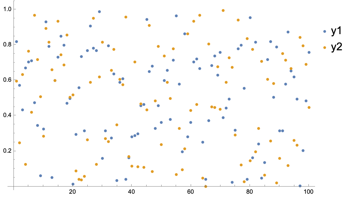
Legends can be added to a plot by specifying the PlotLegends argument. PlotLegends takes either a number of keywords, such as Automatic or "Expressions", or a set of strings that, like in previous examples, can be stylized using the Style function. The strings should be given in the same order as the data was given to be plotted. Further control of the legends placement can be gained by passing the set of strings to the function Placed. Placed takes as its argument first the set of strings used in the legend and then an array of (x, y) positions or keywords such as Above. For \(x, y \ge 1.0\) or \(x,y \le 0.0\) the legend will be placed outside of the frame of the figure.

y2 = RandomReal[{0,1},100]; (* Generate another set of 100 random real numbers between 0 and 1 *)
data2 = Transpose[{x,y2}]; (* Create an (x,y) list of points for plotting *)

ListPlot[{data, data2}, PlotLegends -> Automatic, ImageSize -> Large]	ListPlot[{data, data2}, PlotLegends -> Placed[{Style["y1", 18], Style["y2", 18]}, {1.0, 0.8}], ImageSize -> Large]

Style

Plot Style

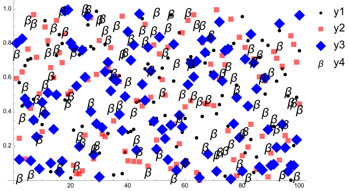
PlotStlye is used to alter the default style or color of your data. The input parameter is typically a set of sets, with each set containing the style options for a set of data. If the number of data sets is longer than the supplied PlotStyle list then the stlye options will simply repeat cyclically. For line data the thickness, color, and style (dashed, dotted, etc) can be set within PlotStyle. For point data we need to add the argument PlotMarkers.

ListPlot[{data, data2, data3, data4}, PlotLegends -> Placed[{Style["y1", 18], Style["y2", 18], Style["y3", 18], Style["y4", 18]}, {1.0, 0.8}], ImageSize -> Large, PlotStyle -> {{Black}, {Red, Opacity[0.6]}, {Blue}}, PlotMarkers -> {{Automatic, Small}, {Automatic, Medium}, {Automatic, Large}, {"\[Beta]", Large}}]	ListPlot[{data, data2, data3}, PlotLegends -> Placed[{Style["y1", 18], Style["y2", 18], Style["y3", 18], Style["y4", 18]}, {1.0, 0.8}], ImageSize -> Large, Joined -> True, PlotStyle -> {{Black}, {Red, Opacity[0.6], Dashed}, {Green, Thick}}]

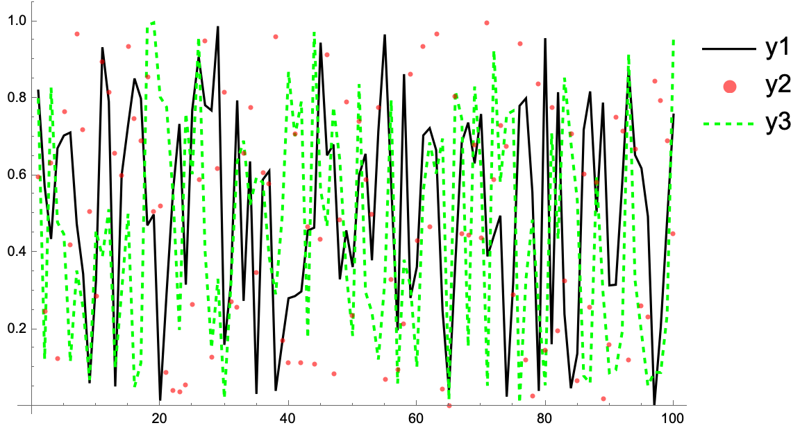The argument Joined was added to plot the first and third/last set of (x, y) point data as lines.

Tick Marks

The tick marks on most figures can be set using either Ticks or FrameTicks and their corresponding style argument TicksStyle and FrameTicksStyle. These arguments behave in similar fashions, although with an annoying argument flip for whether the x-axis argument or the y-axis argument comes first. The Ticks argument also doesn’t work if you want both a left and right axis or a top and bottom axis.

When we use the argument Frame, we need to style the ticks using the two arguments FrameTicks and FrameTicksStyle. FrameTicks can be used to specify the location and label of the major ticks and also change the style of a specific tick mark. FrameTicksStyle can be used to set the style of all the tick marks that haven’t been styled using FrameTicks.

ListPlot[{data}, ImageSize -> Large, Ticks -> {Automatic, {0.0, 0.5, E/4, {1.0, "1.0"}}}, TicksStyle -> Directive[Red, 14]]	ListPlot[{data}, ImageSize -> Large, Frame -> {{True, False}, {True, False}}, FrameTicks -> {{{0.0, {0.5, 1/2}, {Exp[1]/4, E/4, {1.0, 0.00}, Directive[Black, Dashed]}, {1.0, "1.0"}}, None}, {Automatic, Automatic}}, FrameTicksStyle -> Directive[Blue, 14]]

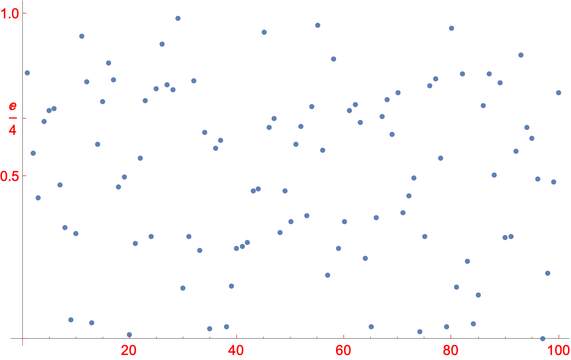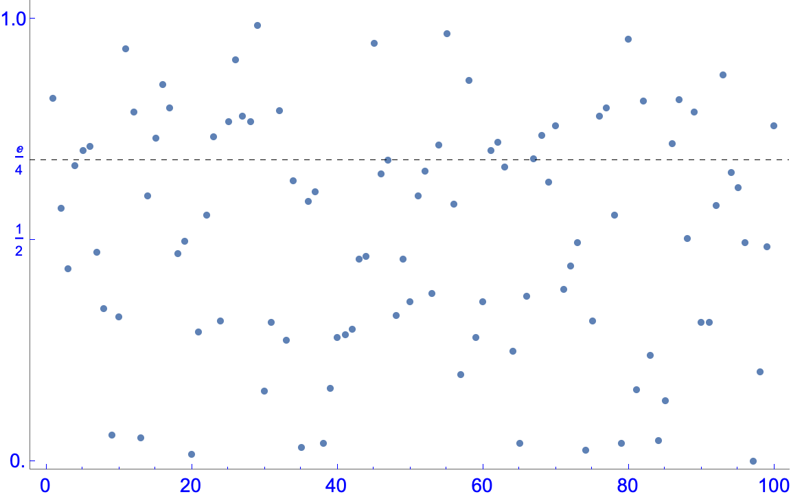Image Size

An image can be resized after it is generated by clicking on it and dragging the orange border that appears. However, style elements do not scale with the size of the plot. If we want to export and save the image we generate it’s important to set an image size and then set the style elements afterwards. If the image size is not large enough it can be hard to get a decent resolution image. The way to do this is to set the argument ImageSize. There are default sizes such as Small, Large, and Full, which uses the full width of the window to generate the image. We can also set the size using a set of pixel sizes, i.e. ImageSize -> {600,400}.

Aspect Ratio

There is no default aspect ratio for a figure. The figure simply fills the space given by ImageSize (whose default is Medium, whatever that means). If ImageSize is set to a specific pixel size then the argument AspectRatio will still affect the plot, but there will be white space around the figure.

ListPlot[{data}, ImageSize -> {600, 400}, AspectRatio -> 1/4]	ListPlot[{data}, ImageSize -> {600, 400}, AspectRatio -> Full]

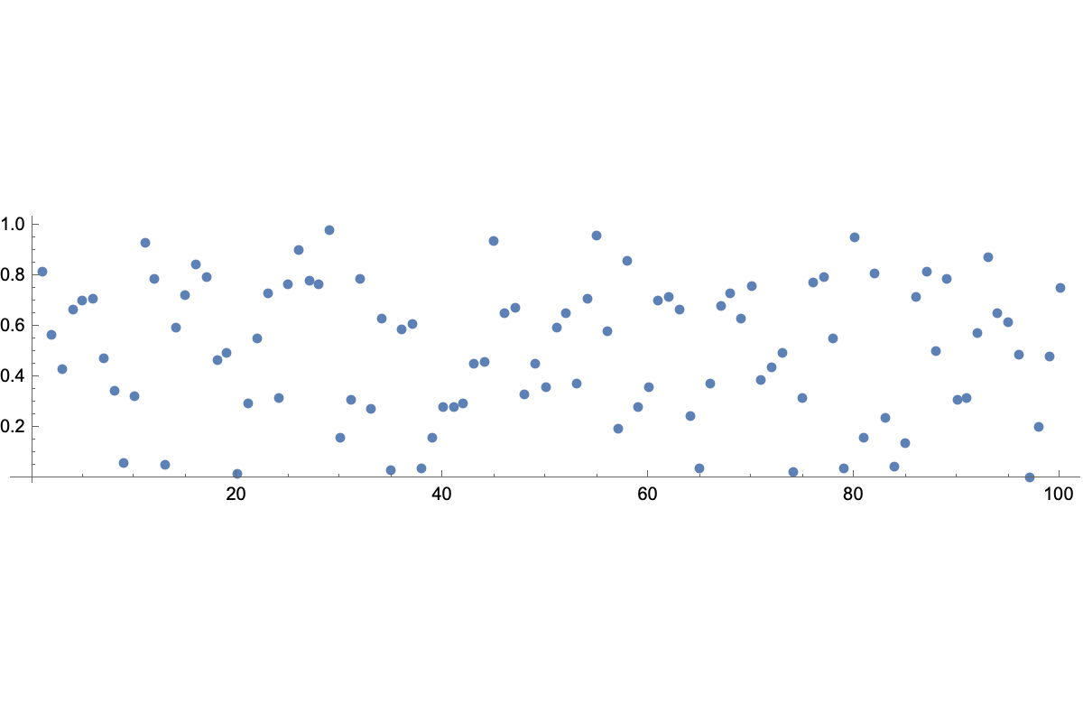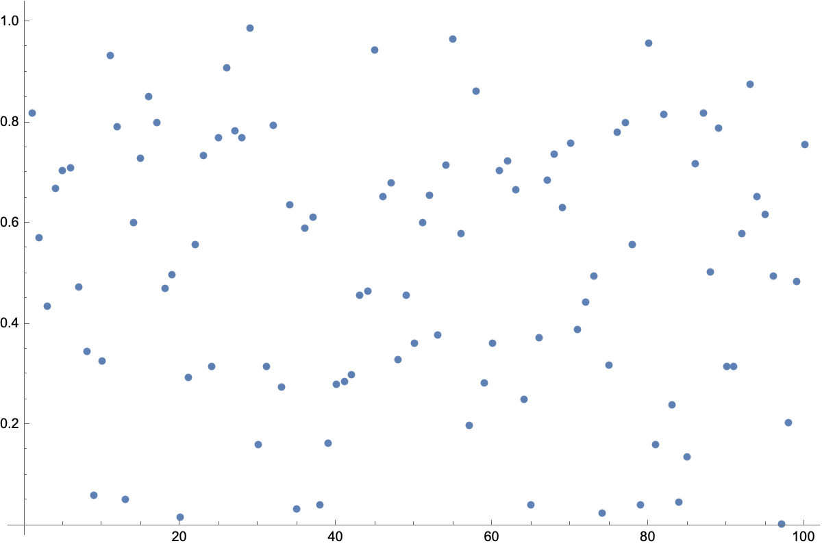Manipulating Parameters

Misc

• use Evaluate to pass multiple values